


MODEL 54e pH/ORP SECTION 6.0
THEORY OF OPERATION
6.9 PID CONTROL (continued)
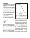
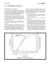
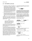
5. The reaction of the system, when graphed, will
resemble Figure 6-2, showing a change in the
measured variable over the change in time. After a
period of time (the process delay time), the meas-
ured variable will start to increase (or decrease)
rapidly. At some further time the process will begin
to change less rapidly as the process begins to sta-
bilize from the imposed step change. It is important
to collect data for a long enough period of time to
see the process begin to level off to establish a tan-
gent to the process reaction curve.
6. When sufficient data has been collected, return the
output signal to its original value using the simulate
test function. Maintain the controller in this manual
mode until you are ready to initiate automatic PID
control, after you have calculated the tuning con-
stants.
Once these steps are completed, the resulting process
reaction curve is used to obtain information about the
overall dynamics of the system. It will be used to cal-
culate the needed tuning parameters of the Model 54e
pH/ORP controller.
NOTE
The tuning procedure outlined below is
adapted from "Instrumentation and
Process Measurement and Control",
by Norman A. Anderson, Chilton Co.,
Radnor, Pennsylvania, ©1980.
Information derived from the process reaction curve
will be used with the following empirical formulas to
predict the optimum settings for proportional and inte-
gral tuning parameters.
Four quantities are determined from the process reac-
tion curve for use in the formulas: time delay (D), time
period (L), a ratio of these two (R), and plant gain (C).
A line is drawn on the process reaction curve tangent
to the curve at point of maximum rise (slope) as shown
in Figure 6-2. The Time Delay (D), or lag time, extends
from "zero time" on the horizontal axis to the point
where the tangent line intersects the time axis. The
Response Time period (L), extends from the end of
delay period to the time at which the tangent line inter-
sects the 100% reaction completion line representing
the process stabilization value. The ratio (R) of the
Response Time period to the Time Delay describes the
dynamic behavior of the system.
In the example, the process Delay Time (D) was four
seconds and the Response Time period (L) was 12
seconds, so:
R = = 3
The last parameter used in the equations is a plant gain
(C). The plant gain is defined as a percent change in the
controlled variable divided by the percent change in
manipulated variable; in other words, the change in the
measured variable (pH, conductivity, temperature) divid-
ed by the percent change in the analog output signal.
The percent change in the controlled variable is
defined as the change in the measured variable (pH,
conductivity, temperature) compared to the measure-
ment range, the difference between the 20 mA (Hi) and
4 (or 0) mA (Lo) setpoints, which you determined when
configuring the analog output.
In the example shown in Figure 6-2:
The percent change in pH was:
x 100% = = 33.3%
The change in the output signal was:
x 100% = 12.5%
So the Plant Gain is:
C = = 2.66
Once R and C are calculated, the proportional and inte-
gral bands can be determined as follows:
Proportional band (%) = P = 286
Integral Time (seconds per repeat) = I = 3.33 D x C
So for the example:
P = = 254%
I = 3.33 (4 sec.) 2.66 = 36 seconds
To enter these parameters, use the procedure detailed
in Section 5.6.
12 seconds
4 seconds
pH2 - pH1
pH “Hi” - pH “Lo”
6 - 4 milliamps
20 - 4
286 (2.66)
3
33.3
12.5
C
R
8.2 - 7.2 pH
9.0 - 6.0 pH
L
D
53